12 Stationarity in Time Series Data
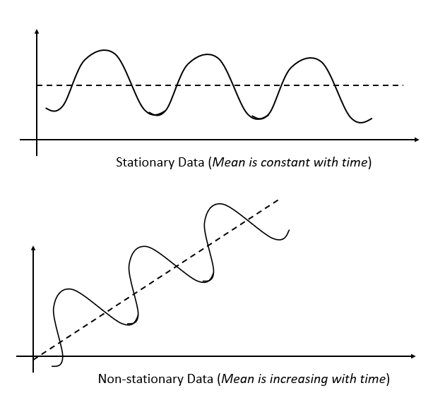
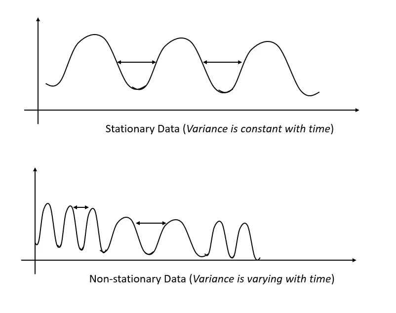
A stationary time series is one whose statistical properties, such as mean, variance, and autocorrelation, do not change over time. In other words, the data fluctuates around a constant mean and has constant variance.


Stationarity ensures that the underlying process generating the data remains stable over time, which is crucial for building predictive models on time series data.
12.1 Types of Stationarity
There are different types of stationarity, including:
- Strict Stationarity: The distribution of the time series does not change over time. This is quite strict, and rarely occurs in real-world data.
- Weak Stationarity (or Second-Order Stationarity): This is the most common type and only requires the mean, variance, and autocorrelation to be constant over time.
12.2 Why Does Stationarity Matter?
In time series analysis, stationarity is a key assumption that greatly influences our choice of which models to use.
For Linear Regression models: while linear regression does not explicitly require stationarity in the data, regression models generally work better with stationary data, particularly if the relationship between the features and the target is assumed to be stable over time.
For ARIMA (Autoregressive Integrated Moving Average) models: ARIMA models require the data to be stationary. If the time series is not stationary, the model’s assumptions break down, and it will not perform well. The “Integrated (I)” part specifically deals with non-stationarity by differencing the data (i.e. subtracting the previous observation from the current one) to make it stationary.
12.3 Testing for Stationarity
Here are some common ways to test for stationarity in time series data:
Visual Inspection: Plot the Data: Plotting the time series can often give a good idea of whether the data is stationary. Look for consistent variance, a constant mean, and no obvious trend or seasonality over time.
Augmented Dickey-Fuller (ADF) Test: The ADF test is a statistical test where the null hypothesis is that the data has a unit root (i.e. is non-stationary). If the p-value is below a certain threshold (e.g. 0.05), we can reject the null hypothesis, indicating that the series is stationary. In Python, we can use the
adfullerfunction fromstatsmodels:
from statsmodels.tsa.stattools import adfuller

result = adfuller(time_series)
print(f"ADF Statistic: {result[0]}")
print(f"P-value: {result[1]}")- KPSS Test (Kwiatkowski-Phillips-Schmidt-Shin): the KPSS test is another test for stationarity, but its null hypothesis is the opposite of the ADF test. In KPSS, the null hypothesis is that the series is stationary. A low p-value indicates non-stationarity. In Python, we can use the
kpssfunction fromstatsmodels:
from statsmodels.tsa.stattools import kpss

result = kpss(time_series)
print(f"KPSS Statistic: {result[0]}")
print(f"P-value: {result[1]}")- Rolling Statistics: another simple method is to calculate the rolling mean and variance over time. If these values change significantly over time, the series is likely non-stationary.
rolling_mean = time_series.rolling(window=12).mean()
rolling_std = time_series.rolling(window=12).std()
12.3.1 Transformations to Achieve Stationarity
If your data is non-stationary, here are a few common techniques to make it stationary:
Differencing: Subtracting the previous value from the current value to remove trends.
Logarithmic Transformation: Taking the logarithm of the data can help stabilize variance.
De-trending: Remove trends either by subtracting a moving average, or fitting a regression model and subtracting the predicted trend.
Seasonal Decomposition: If there’s seasonality, we can decompose the time series into trend, seasonality, and residual components and work with the residuals.
