Generalization

In machine learning, generalization refers to the model’s ability to perform well on unseen data, rather than simply memorizing specific patterns in the training set. A model that generalizes well captures the underlying structure of the data and performs accurately when exposed to new inputs. Achieving good generalization is one of the primary goals in machine learning.

Let’s discuss key concepts related to generalization, including the trade-off between overfitting and underfitting, the importance of splitting datasets into training and testing sets, and the role of cross-validation in evaluating model performance.

Bias vs Variance

In the context of generalization, bias and variance represent two types of errors that can affect a model’s performance.

Bias refers to errors introduced by overly simplistic models that fail to capture the underlying patterns in the data. A high-bias model makes strong assumptions about the data, resulting in consistently poor predictions on both the training and test sets.

On the other hand, variance refers to errors caused by overly complex models that fit the training data too closely, capturing noise along with the signal. This leads the model to perform well on the training data, but poorly on unseen test data.

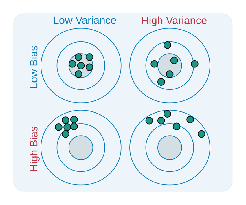
Illustration of bias vs variance, using a bull’s eye. Source: Gudivada 2017 Data.

Using an analogy of darts on a bull’s eye, low bias means the predictions are accurately centered around the optimal target, whereas high bias means the attempts are consistently off the mark. Low variance means all the attempts are concentrated in a specific region, whereas high variance means the attempts are spread out over a wider region. The goal is to achieve results which are accurate (with low bias), and consistent (with low variance).

Overfitting vs Underfitting

Overfitting

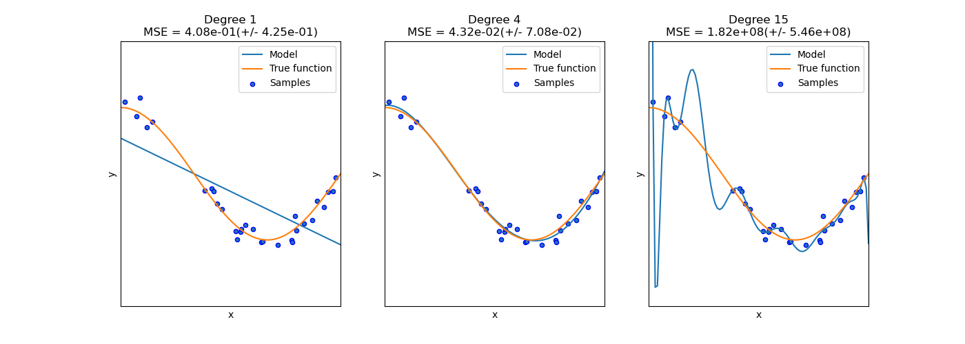
Overfitting occurs when a model is too complex and learns not only the underlying patterns but also the noise and random fluctuations in the training data. An overfitted model performs very well on the training data but fails to generalize to unseen data. This results in poor performance on the test set, as the model struggles to adapt to new inputs that do not perfectly match the training data.

In technical terms, overfitting happens when a model has low bias but high variance. The model fits the training data very closely, but any small changes in input data lead to significant variations in the output predictions.

Common causes of overfitting include:

Using a model that is too complex for the given data (e.g. deep neural networks on small datasets).
Training the model for too long without proper regularization.
Using too many features or irrelevant features.

Underfitting

Underfitting occurs when a model is too simple to capture the underlying structure of the data. An underfitted model performs poorly on both the training data and the test data because it fails to learn the important relationships between input features and output labels.

In technical terms, underfitting happens when a model has high bias but low variance. The model is too rigid, making overly simplistic predictions that do not adequately capture the complexities of the data.

Common causes of underfitting include:

Using a model that is too simple for the task at hand (e.g. linear regression for non-linear data).
Not training the model long enough or with sufficient data.
Using too few features or ignoring important features.

Finding a Balance

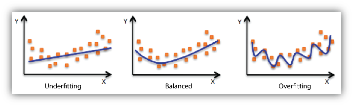
The challenge in machine learning is to find the right balance between bias and variance, often called the bias-variance tradeoff, in order to achieve good generalization. A model with the right balance will generalize well to new data by capturing the essential patterns without being too sensitive to specific details in the training data.

Three different models, illustrating trade-offs between overfitting and underfitting. Source: AWS Machine Learning.

Data Splitting

When building a machine learning model, it is important to evaluate its performance on data that the model has not seen during training. This ensures that the model is not overfitting and can generalize to new data.

Two-way Splits

To keep some of the data unseen, we split the available data into training and testing datasets:

Training set: This is the portion of the data that the model is trained on. The model learns patterns and relationships in the data using this set.
Testing set: This is a separate portion of the data that the model has never seen before. After training the model, the test set is used to evaluate its generalization ability.

A common strategy for splitting the data is the train-test split, where a portion of the data (often 70-80%) is reserved for training, and the remaining (20-30%) is used for testing. This approach allows us to estimate the model’s performance on unseen data.

Two-way split (training and test sets). Source: Google ML Concepts.

Three-way Splits

In practice, we often use a validation set in addition to the training and test sets, particularly when fine-tuning a model’s hyperparameters. The validation set allows us to adjust and optimize the model’s hyperparameters across multiple runs without ever exposing the model to the test set. This reduces the risk of overfitting to the test data.

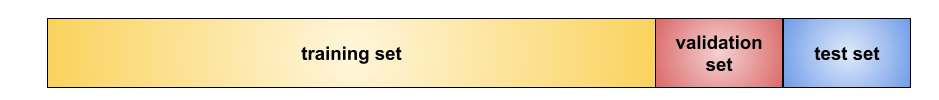
Three-way split (training, validation, and test sets). Source: Google ML Concepts.

After training the model on the training data, we evaluate its performance on the validation set. This process can be repeated iteratively, adjusting hyperparameters and retraining the model until the performance is satisfactory.

Workflow using validation set. Source: Google ML Concepts.

Once we believe the model is well-optimized, we use the test set to evaluate its true generalization ability on unseen data. By limiting the model’s exposure to the test set until the final evaluation, we ensure that the test results provide an unbiased estimate of real-world performance.

Cross Validation

With cross validation, instead of relying on a single training or validation set, we use multiple validation sets to improve the model’s robustness and reduce the risk of overfitting.

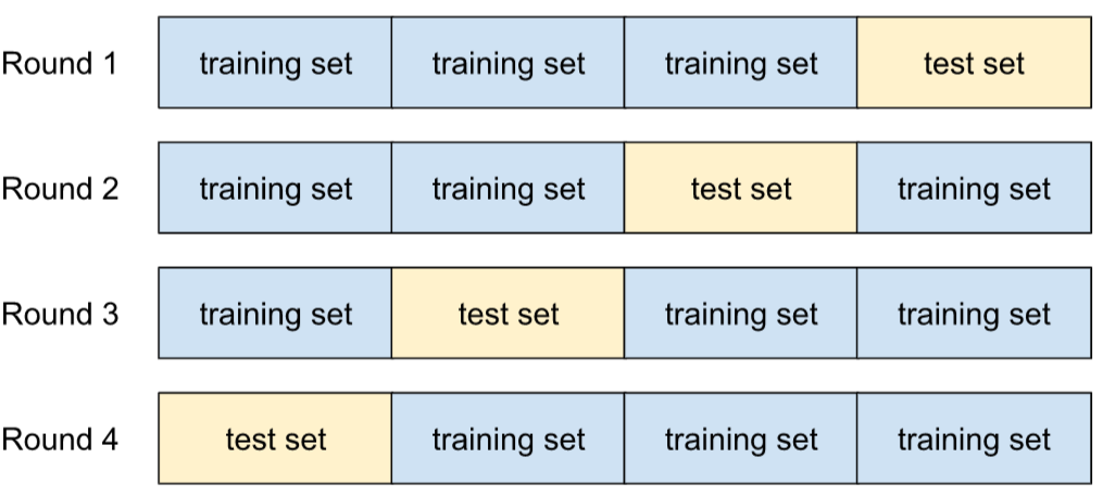
In K-fold cross validation, the dataset is divided into several subsets or “folds”, and the model is trained and validated on different subsets of the data in each iteration. This provides a more comprehensive understanding of the model’s performance across various data splits, making it less sensitive to any specific partitioning.

Cross validation is especially valuable when fine-tuning model hyperparameters, as it prevents overfitting to a specific validation set or the test set by providing a more generalized evaluation before the final test set assessment.

How to Split

This section provides some practical methods for splitting data in Python.

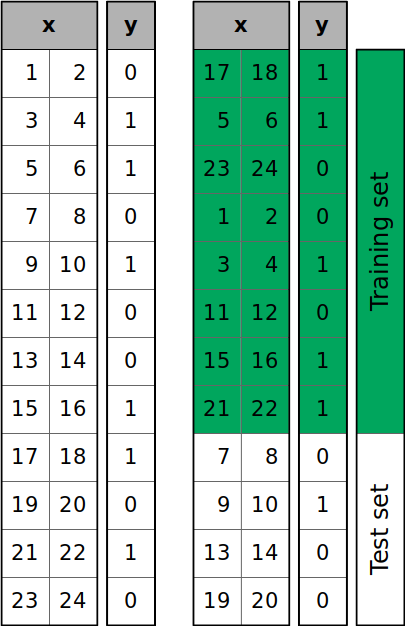
Shuffled Splits

In most machine learning problems, we typically perform a shuffled split, where the order of the data is randomized before partitioning it into training and testing sets. This randomization helps ensure the distribution in the training set closely resembles that of the test set, reducing potential biases that could skew model performance.

Shuffled train/test split. Source: Real Python.

One major benefit of shuffling is that it helps prevent sequential bias, which occurs when the order of the data affects the model’s ability to generalize. Sequential bias can lead to inconsistencies in predictions, especially if certain patterns or trends exist in the sequence of the data. For example:

In a regression problem such as predicting student grades based on study hours, imagine the dataset is originally sorted with the highest-performing students listed first and the lowest performers listed last. If we split this data sequentially, the training set would contain only high achievers, leaving the model unprepared for students with lower performance, resulting in poor predictions.
Similarly, in a classification task, such as distinguishing between images of dogs and cats, if the data is sequentially ordered by class (e.g. all dog images first, followed by cat images), a non-shuffled split could lead the model to train mostly on one class, causing it to over-predict that class and fail to generalize properly to the other.

By shuffling the data, we ensure a more representative sample in both the training and testing sets, reducing the risk of biased or inaccurate predictions.

One common way of implementing a shuffled two-way split in Python is to leverage the train_test_split function from sklearn:

from sklearn.model_selection import train_test_split

x_train, x_test, y_train, y_test = train_test_split(x, y, test_size=0.2,
                                                          random_state=99)
print("TRAIN:", x_train.shape, y_train.shape)
print("TEST:", x_test.shape, y_test.shape)

When using the train_test_split function, we pass in the features (x) and labels (y), specify a test_size either as a fraction (e.g. 0.2 for 20% of the data) or as an absolute number of samples. We also supply a random_state to enable reproducibility. As a result, we obtain four different datasets: features and labels for training and testing, respectively.

Reproducibility

The random_state parameter ensures that the same random shuffling and splitting occurs every time you run the code. You can choose any integer, but once it’s set, subsequent executions will produce the same split. This enables consistent, reproducible results, and allows us to more accurately compare model performance across multiple runs. Without consistency of splits, results may differ slightly due to random variations in the data split, potentially confounding differences between runs and leading to misleading model evaluations.

Sequential Splits for Time-series Forecasting

Most of the time we want to shuffle the data when splitting, however this may not be the case with time-series data.

If we shuffle the data when performing a train/test split for time-series forecasting, several critical issues arise due to the nature of time-dependent data:

Data Leakage: Shuffling can lead to training on future data points and testing on past ones, which is unrealistic in real-world forecasting. This would allow the model to “see the future,” resulting in overly optimistic performance during evaluation. In practice, you’ll never have access to future data when making predictions.
Loss of Temporal Structure: Time series data inherently depends on the order of observations. Shuffling breaks the sequence and removes temporal relationships, leading the model to learn patterns that don’t reflect how time-dependent data actually behaves. This can distort predictions and diminish the model’s forecasting ability.
Unreliable Performance Metrics: If the model is trained on future data, performance metrics like accuracy or MSE will be unrealistically high, but once deployed, the model’s performance will significantly degrade as it won’t have access to future data at inference time.

Instead of shuffling time series data, we can split based on time, using methods like sequential splits, or time-based cross-validation, ensuring that the training set only contains past data relative to the test set.

To implement a sequential split, assuming your data is sorted by date in ascending order, pick a cutoff date, and use all samples before the cutoff in the training set, and samples after the cutoff date in the test set. This ensures the model can’t rely on data from the future when making predictions for the test set.

training_size = 0.8
cutoff = round(len(df) * training_size)

x_train = x.iloc[:cutoff] # all before cutoff
y_train = y.iloc[:cutoff] # all before cutoff

x_test = x.iloc[cutoff:] # all after cutoff
y_test = y.iloc[cutoff:] # all after cutoff

print("TRAIN:", x_train.shape, y_train.shape)
print("TEST:", x_test.shape, y_test.shape)

For your reference, here is a reusable helper function containing the same sequential split logic:

def sequential_split(x, y, training_size=0.8, test_size=None):
    training_size = 1 - test_size if test_size
    assert len(x) == len(y)
    cutoff = round(len(x) * training_size)

    x_train = x.iloc[:cutoff] # all before cutoff
    y_train = y.iloc[:cutoff] # all before cutoff
    x_test = x.iloc[cutoff:] # all after cutoff
    y_test = y.iloc[cutoff:] # all after cutoff

    return x_train, x_test, y_train, y_test


x_train, x_test, y_train, y_test = sequential_split(x, y)
print("TRAIN:", x_train.shape, y_train.shape)
print("TEST:", x_test.shape, y_test.shape)